

In project risk analysis, statistical distributions are an integral component of how we model both uncertainties and risk impacts, and are often misunderstood by the uninitiated. So let’s take a look at how we use statistical distributions to model probability.
Here is a simple example. Look at this police lineup. All these people have different heights:
1. 5’10”
2. 6’3”
3. 5’7”
4. 5’11”
5. 5’5”

Let’s group these numbers:
Group 1: From 5’0 to 5’6” – 1 person
Group 2: From 5’6” to 6’0” – 3 people
Group 3: From 6” to 6’6” – 1 person
Now we can present these groups on a chart: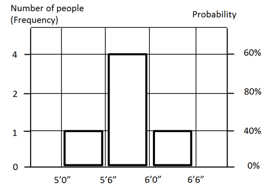
Horizontal axis of this chart shows the actual value, which it in this case height of the person. The left vertical axis shows the number of people for the range. It is called the frequency. The right vertical axis shows the probability. Probability is the chance that something will happen or occurred. In our case total number of people is 5. Number of people between 5’6” and 6’0” is 3. Therefore, probability will be 3/5 = 60%. It means that based on this sample of people, probability that height will be between 5’6” and 6’0” is 60%.
The chart on is called Frequency Histogram. It was first introduced by Karl Pearson – British mathematician and statistician. This histogram and data table represents a statistical or probability distribution or relationship between data samples and their probability of occurrence. It is important to remember that distribution can be applied to any ranges of values, which can be an input or an output ( results), of analysis.
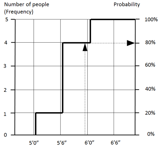
The data in the histogram can be drawn differently. We can sum up number of samples, or probabilities from the left to right and present the result as a line (see below). This is called a Cumulative Probability chart. What is the value of this view of the data? Using cumulative probability plots it is easy to determine how values are associated with probability. Just select a value on the horizontal axis then draw a vertical line until it crosses the cumulative probability line and you will find the probability and frequency associated with a selected value. In our example, there is an 80% probability that a person’s height will be less or equal to 5’11”. Cumulative probability plots are useful when you compare different uncertain variables, for example, when you compare multiple scenarios.
Statistical Parameters
Each statistical distribution has several statistical parameters, which are useful to describe properties of the distribution. The parameter that first comes to mind when we talk about distributions is the mean, or average value. In our example, the mean equals 5’10”. However, mean does not tell us how wide statistical distribution is. It is like the average body temperature in the hospital, which is always very close to normal because while someone may have a fever, bodies in the morgue are dead and cold.
It is possible to measure the width of the distribution using different values around the extremes. However, in most real life situations, these measures can be misleading. For example, the tallest man in medical history was Robert Wadlow from Alton, Illinois. He was 8’11.1” (2.72 m). Chandra Bahadur Dangi from Nepal was shortest adult person. He was 21.5” (54.6 cm). The difference in height between tallest and shortest people is 217.4 cm or just over 7’. But this range may not be very representative for the analysis that you are doing as there are only few people in the world whose heights are at these extremes. Because of this, we prefer to use other statistical parameters that can be used to address this problem, variance and standard deviation.
Variance – a measure of how widely dispersed the values are in a distribution, and thus is an indication of the risk of the distribution. It is calculated as the average of the squared deviations about the mean. The variance gives disproportionate weight to outlying values that are far from the mean.
One of the most important parameters for understanding statistical distribution is standard deviation – a measure of how widely dispersed the values are in a distribution. For example, if a project’s task duration is greater than the standard deviation, then wider statistical distributions and more uncertainties are associated with the task duration. It is one of the most important parameters of statistical distribution. Standard deviation equals the square root of the variance. Semi standard deviation is a measure of dispersion for the values falling below the mean or another target value. Semi standard deviation is calculated the same way as standard deviation, except only samples below mean or target values are used in the calculation.
Another statistical parameter is kurtosis. Kurtosis is a measure of the flatness or peaked nature of a distribution relative to a normal distribution. A parameter called skewness is a measure of the degree of asymmetry of a distribution around its mean. If the distribution is skewed to the left, it will have a positive skewness. If it is skewed to the right, it will have a negative skewness.
Schedule risk analysis software packages usually present these statistical parameters as the results of Monte Carlo simulations.
Percentiles are another type of statistical parameter. It is a value on a scale of zero to 100 that indicates the percentage of a distribution that is equal to or below this value. A value in the 90th percentile (sometimes defined as P90) is a value equal to or lower than 90 percent of all other values in the distribution. Here is an example. You have the following 10 values:
20, 22, 10, 5, 34, 40, 48, 7, 32, 49
To calculate percentiles, all samples need to be sorted:
5, 7, 10, 20, 22, 32, 34, 40, 48, 49
Number 22 is P50 because there are 5 values below or equal or below 22. Interestingly, P50 is not necessarily the mean, which in this case is 26.7.
So, statistical distributions can present actual data, but also represent models of expected probabilities for specific parameters during projects. We use these statistical distributions in two ways: to model uncertain inputs for cost and schedule, and to generate probabilistic outcomes that provide statistical analysis measures of project parameters. If you would like to find out more information about how to use statistical distributions in your project risk analysis, please visit our YouTube channel and watch this playlist that provides more detailed information and practical examples on the use of statistical distributions in Monte Carlo simulations.